Computation of Representation Topology Divergence (RTD)
Example #1
| 1) |
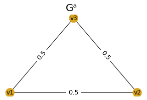
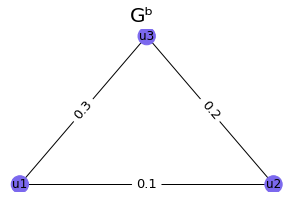
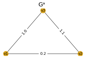
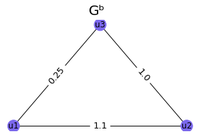
Let's consider two graphs Ga and Gb. |
| 2) |
Corresponding H0 diagrams (built by Ripser++ package) look in the following way 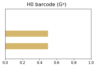
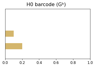
Note that Ripser doesn't draw infinity H0 bar, this is why the number of bars is less than the number of the connected components by one. |
| 3) |
|
| 4) |
|

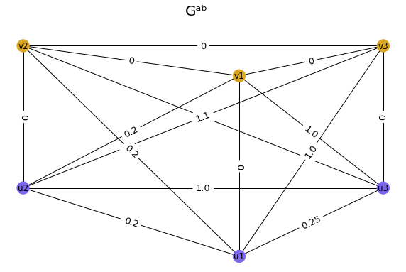
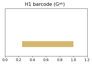
| 5) |
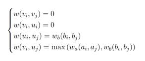
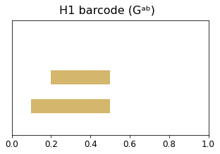
Note that by definition, all edges between the nodes, corresponding to Ga graph (denoted as v1, v2, v3) and between nodes with the same indices have zero weights; all edges between the nodes, corresponding to Gb graph (u1, u2, u3) have the same weight as they had in Gb graph; all other edges have weight 0.5 because when we get a maximum of two edges - one from graph Ga and one from graph Gb, we always get this value. H1 barcode of this new graph, calculated with Ripser++, looks in the following way |
|
| 6) |
Now we can calculate RTD(Ga, Gb) as the sum of the bars of this barcode, that is equal to 0.7. |
|
Now let us explain why does H1 barcode for this graph look as it looks.
|
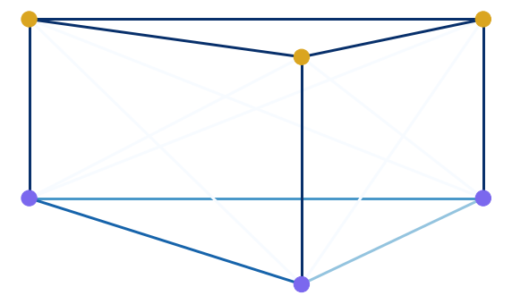
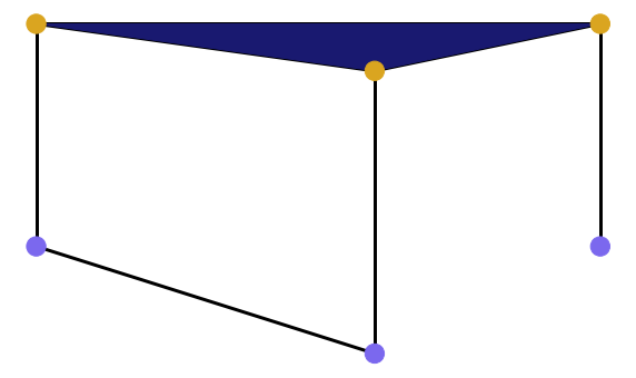
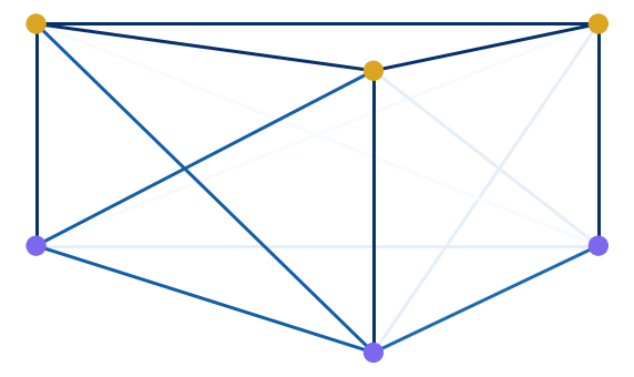
To make it more clear, we will now represent weights of Gab visually, using colors. The darkest edges have the mimimum weight, equal to 0, and the lightest ones have the maximum weight, equal to 0.5. |
|
|
Let's now see, what will happen, if we will take into account only edges with weight less than 0.1 (in other words, if we filter our graph by some threshold 0 < ε < 0.1). Also recall that, strictly speaking, we calculate a barcode not from the graph Gab itself, but from the slightly bigger constructions, called a flag complexes, associated with the graph on every threshold ε. To construct a flag complex upon our graph for the current threshold ε, we do the following: we span a simplex (triangle, tetrahedron etc) on those vertices, which form a clique for the current ε. Since edges (v1, v2), (v2, v3) and (v3, v1) have zero weights, they remain in our construction for every ε > 0, and thus they always form a clique, which we fill in with a triangle. There are no cycles in this complex, so, using the language of algebraic topology, we say that H1 homology group is trivial for ε < 0.1. Thus there is no bars between these values. |
|
|
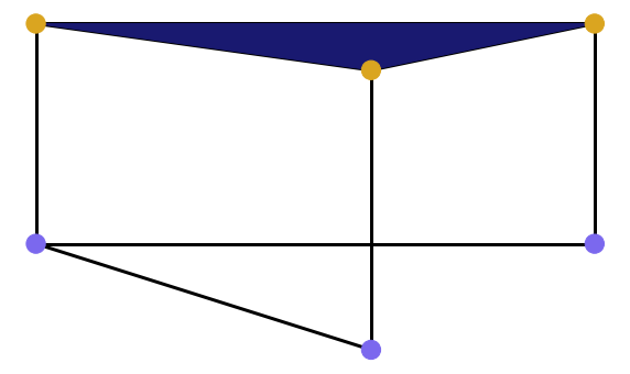
For 0.1 ≤ ε < 0.2 we include an edge with the weight 0.1 and get such picture. There is one cycle. Algebraic topologists experss it by saying that H1 homology group is one dimensional for 0.1 ≤ ε < 0.2. It is illustrated by the lower bar on the barcode, which starts at ε = 0.1. |
|
|
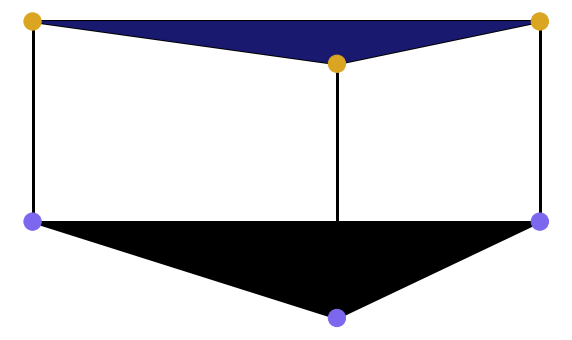
Now let's see what happens for 0.2 ≤ ε < 0.3, when we add one more edge. One more cycle appears, so we start one more bar from the point 0.2. In the same time, the previous cycle still persists, so the previous bar also continues. H1 homology group is now two dimensional. |
|
|
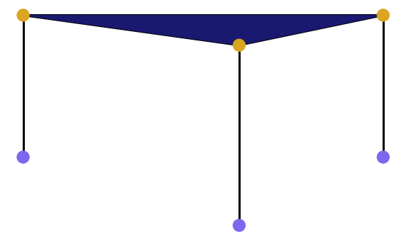
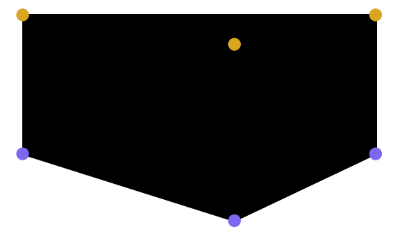
An interesting thing happens when we add the edge with the weight 0.3. At first, the lower three vertices now also form a clique, so we add a new triangle. At second, a new loop appear, but we don't count it for a barcode, because it can be represented as a sum of the two other loops. Thus, formally speaking, H1 remains two dimensional, and we further continue two bars. |
|
|
Finally, when we reach the threshold 0.5, all edges appear in the graph, and it all turn into one big clique. In the corresponding flag complex, all cycles dissapear. Thus all bars end on the point 0.5. The clique is actually filled in with the multi-dimensional simplex, but we drew it's two dimensional projection for clarity. |
|
Example #2
| 1) |
Now let's calculate RTD between following two graphs |
|
|
| 2) |
Here is how Gab looks like in this case: |
|
| 3) |
H1 barcode of this new graph, calculated with Ripser++, looks in the following way |
|
| 4) |
There is only one bar, so RTD(Ga, Gb) is equal to the length of this bar, which is 0.75. |
|
Now let us explain why does H1 barcode for this graph look as it looks.
|
To make it more clear, we will now represent weights of Gab visually, using colors. The darkest edges have the mimimum weight, equal to 0, and the lightest ones have the maximum weight, equal to 0.5. |
|